Fluid Kinematics
In fluid mechanics one describes the properties of the system under consideration in terms of fields - mathematical objects that assign values to each point in space, hence characterising some local physical property such as pressure, density or the velocity.
When evaluating the local dynamics within the fluid, it will however not be sufficient to deal with single points only. In the continuum limit, single points do not possess any mass and have therefore no physical significance. Instead, one always has to take into account finite volume elements, also called control volumes which possess a finite mass and are subject to external forces.
Say, one wants to evaluate the fluid kinematics in the vicinity of some point $\vec{r}$. This vicinity is given by a small volume $\delta V$ which is made up of some set of points \begin{align} \vec{r}' = \vec{r} + \delta \vec{r} = \begin{pmatrix} x \\ y \\ z \end{pmatrix} + \begin{pmatrix} \delta x \\ \delta y \\ \delta z \end{pmatrix} \end{align} with $\left| \delta \vec{r} \right|$ being small enough such that the fluid characteristics do not vary too much within $\delta V$.
Under this assumption the velocity field within $\delta V$ can be described by a linear approximation. For one dimension one finds: \begin{align} v_x \left( \vec{r} + \delta\vec{r} \right) &\approx v_x (\vec{r}) + \delta x \left. \frac{\partial v_x}{\partial x} \right|_\vec{r} + \delta y \left. \frac{\partial v_x}{\partial y} \right|_\vec{r} + \delta z \left. \frac{\partial v_x}{\partial z} \right|_\vec{r} \\[2ex] &= v_x(\vec{r}) + \left. \left( \delta \vec{r} \cdot \nabla \right) v_x \right|_\vec{r} \end{align} If this expression is extended to three dimensions, one receives \begin{align} \vec{v} \left( \vec{r} + \delta \vec{r} \right) &\approx \vec{v} \left( \vec{r} \right) + \left( \delta \vec{r} \cdot \nabla \right) \vec{v} (\vec{r}) \\ &= \vec{v} \left( \vec{r} \right) + \xi \, \delta \vec{r} \label{eq:lin-approx-v} \end{align} with \begin{align} \xi = \begin{pmatrix} \partial_x v_x & \partial_y v_x & \partial_z v_x \\ \partial_x v_y & \partial_y v_y & \partial_z v_y \\ \partial_x v_z & \partial_y v_z & \partial_z v_z \end{pmatrix} \end{align} being the Jacobian matrix (representing a second-order tensor) which contains all spatial derivatives of the velocity vector $\vec{v}$ (evaulated at $\vec{r}$) and $\partial_i$ being a shortcut for the partial derivative with respect to the spatial variable $i$.[1]
The properties of the velocity field within $\delta V$ are completely determined by the vector $\vec{v}(\vec{r})$ and the velocity gradient tensor $\xi$.
Fundamental Types of Motion
The general kinematics given by $\vec{v}(\vec{r})$ and $\xi$ can be thought of as being a composition of some fundamental types of motion, as we will see in a moment:
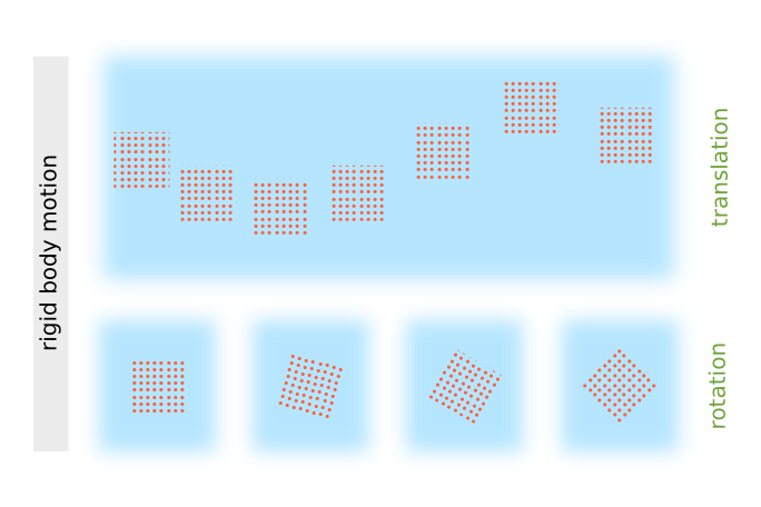
Rigid Body Motion
The velocity vector $\vec{v}(\vec{r})$ corresponds to a uniform translation (like as a rigid body) of $\delta V$ as a whole.
The velocity gradient tensor $\xi$ is a square matrix (3x3) that can be decomposed into a symmetric and an antisymmetric part: \begin{align} \xi_{ij} = \underbrace{ \frac{1}{2} \left( \xi_{ij} + \xi_{ji} \right) }_{\xi_{ij}^{(s)}} + \underbrace{ \frac{1}{2} \left( \xi_{ij} - \xi_{ji} \right) }_{\xi_{ij}^{(as)}} \end{align} The first term $\xi_{ij}^{(s)}$ remains unchanged when switching the indices $i$ and $j$ (hence being symmetric) while in the second term $\xi_{ij}^{(as)}$ the overall sign would switch under exchange of $i$ and $j$ (hence being antisymmetric). However, the sum of both just yields $\xi_{ij}$, so this is a valid decomposition.
Antisymmetric Part
In the antisymmetric part the diagonal elements vanish all together since \begin{align} \xi_{ii}^{(as)} = \frac{1}{2} \left( \xi_{ii} - \xi_{ii} \right) = 0 . \end{align} Thus one is left with the six off-diagonal elements, but only three of them are independent of each other because: \begin{align} \xi^{(as)}_{ij} = - \xi^{(as)}_{ji} \end{align} When being written out explicitly, this reads: \begin{align} \xi^{(as)} = \frac{1}{2} \cdot \begin{pmatrix} 0 & \partial_y v_x - \partial_x v_y & \partial_z v_x - \partial_x v_z \\ \partial_x v_y - \partial_y v_x & 0 & \partial_z v_y - \partial_y v_z \\ \partial_x v_z - \partial_z v_x & \partial_y v_z - \partial_z v_y & 0 \end{pmatrix} \end{align} At this point one may notice that the remaining elements represent components of the vorticity vector $\vec{\omega}$ which is defined as the curl of the velocity field: \begin{align} \vec{\omega} := \nabla \times \vec{v} = \begin{pmatrix} \partial_y v_z - \partial_z v_y \\ \partial_z v_x - \partial_x v_z \\ \partial_x v_y - \partial_y v_x \end{pmatrix} =: \begin{pmatrix} \omega_x \\ \omega_y \\ \omega_z \end{pmatrix} \end{align} Furthermore, when the antisymmetric part $\xi^{(as)}$ is applied to a small displacement vector $\delta \vec{r}$ as in eq. \eqref{eq:lin-approx-v}, one obtains: \begin{align} \xi^{(as)} \delta\vec{r} &= \frac{1}{2} \cdot \begin{pmatrix} 0 & - \omega_z & \omega_y \\ \omega_z & 0 & - \omega_x \\ - \omega_y & \omega_x & 0 \end{pmatrix} \begin{pmatrix} \delta x \\ \delta y \\ \delta z \end{pmatrix} \\ &= \frac{1}{2} \cdot \begin{pmatrix} \omega_y \delta z - \omega_z \delta_y \\ \omega_z \delta x - \omega_x \delta_z \\ \omega_x \delta y - \omega_y \delta_x \end{pmatrix} \\ & = \underbrace{ \frac{1}{2} \cdot \vec{\omega} }_{\vec{\Omega}} \times \delta \vec{r} \end{align} Thus, the antisymmetric part $\xi^{(as)}$ describes a fluid motion that corresponds to a local rigid body rotation with an angular frequency $\Omega = \frac{\omega}{2}$ which is equal to half of the local vorticity $\omega$.[2] (for a derivation see the subsection below)
The velocity vector $\vec{v}$ and the antisymmetric part $\xi^{(as)}$ of the velocity vector gradient tensor account for the local rigid-body-like motion. $\vec{v}$ describes rigid translation, while $\xi^{(as)}$ comprises rigid rotation.
Relation between Vorticity and Rigid Body Rotation
The rotation of a rigid body (located at $\vec{r}$) can be described by a vector $\vec{\Omega}$ where $\left| \vec{\Omega} \right|$ is the angular velocity of the rotation and direction given by $\vec{\Omega}$ points along the axis of rotation. Then the velocity at a point $\vec{r} + \delta \vec{r}$ within the rigid body due to the rotation is: \begin{align} \vec{v} \left( \vec{r} + \delta \vec{r} \right) = \vec{\Omega} \times \delta\vec{r} \end{align} vorticity was defined as the curl of the velocity, thus in the case of rigid body rotation the vorticity is \begin{align} \vec{\omega} &= \nabla \times \left[ \Omega \times \delta \vec{r} \right] \\ &= \vec{\Omega} \cdot \left( \nabla \cdot \delta\vec{r} \right) - \left( \nabla \cdot \vec{\Omega} \right) \cdot \delta\vec{r} \\ &= 3\vec{\Omega} - \vec{\Omega} = 2 \vec{\Omega} \end{align}
For the evaluation of the triple vSo we are left with the symmetric part ?(s) of the velocity gradient tensor ? only and we already concluded that it describes pure strain motion without bulk translation/rotation.ector product the so called BAC-CAB rule was used. However, due to the presence of the derivative operator $\nabla$ the order of the expressions matters and has to be modified slightly ($\nabla$ does not affect the constant vector $\vec{\Omega}$ but it acts on $\delta\vec{r}$ and thus $\delta \vec{r}$ has to stay on the right of $\nabla$).
Thus, a locally constant vorticity $\vec{\omega}$ corresponds to a rigid body rotation with a rotation vector: \begin{align} \vec{\Omega} = \frac{1}{2} \cdot \vec{\omega} \end{align}
Non-Rigid Motion: Strain
So one is left with the symmetric part $\xi^{(s)}$ of the velocity gradient tensor. According to the previous reasoning, it must describe the non-rigid part of the motion, i.e. a motion which produces only relative displacements (strain) of adjacent fluid particles without further translation/rotation of $\delta V$ as a whole.
Now one can apply some knowledge from linear algebra: Real symmetric matrices are orthogonally diagonalisable, i.e. there is an orthogonal basis (of eigenvectors) in which the matrix has diagonal form. So in this basis the matrix reads: \begin{align} \xi^{(s)} = \begin{pmatrix} \xi^{(s)}_{11} & 0 & 0 \\ 0 & \xi^{(s)}_{22} & 0 \\ 0 & 0 & \xi^{(s)}_{33} \end{pmatrix} \end{align} This can be further decomposed into an isotropic part \begin{align} \xi^{(s1)}_{ii} :&= \frac{1}{3} \cdot \left( \xi^{(s)}_{11} + \xi^{(s)}_{22} + \xi^{(s)}_{33} \right) \\ &= \frac{1}{3} \cdot \text{Tr} \left( \xi^{(s)} \right) \end{align} that accounts for pure volume change (uniform expansion or compression) and the remaining traceless part \begin{align} \xi^{(s2)} = \xi^{(s)} - \xi^{(s1)} \end{align} that comprises an ellipsoidal stretching without change in volume.[3]
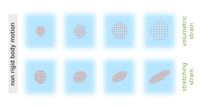
Summarising this article, fluid motion can be decomposed into some fundamental types of motions: Rigid body-like motion that accounts for translation and pure rotations as well as non-rigid strain that can be either volumetric (change of volume) or stretching (change of shape).
References
| [1] | Fluid Mechanics Academic Press 2002 (p. 61) |
| [2] | Fluid Mechanics Academic Press 2002 (p. 62) |
| [3] | Fluid Mechanics Academic Press 2002 (p. 62f.) |